Jeff Rubin ASPO-USA 2010 Peak Oil Conference

Jeff Rubin ASPO-USA 2010 Peak Oil Conference from ASPO-USA on Vimeo.

Jeff Rubin (born August 24, 1954) is a Canadian economist and author. He is a former chief economist at CIBC World Markets.

Rubin graduated from McGill University with a Masters in Economics after completing his Economics B.A. at University of Toronto. He began his career as an economist at the Ontario Government Treasury Department where he was responsible for projecting future interest rates. He moved on to the brokerage firm Wood Gundy which was taken over by CIBC and became first CIBC Wood Gundy and then CIBC World Markets. He has accurately predicted fluctuations in interest rates and the value of the Canadian dollar. In the early 1990s he came to prominence projecting a major decline in the Ontario real estate market. He was one of the first economists to accurately predict soaring oil prices back in 2000 and is now a popular commentator on oil depletion and its economic repercussions. Jeff writes a blog published every Wednesday for The Globe and Mail newspaper. He is an avid fisherman known for exotic trips to northern Canada (B.C. and Yukon) who frequently uses fishing analogies and references to his own fishing experiences, in his writings.^[1]

Rubin had worked at CIBC World Markets and its predecessors since 1988, and served as chief economist from 1992 to 2009, when he resigned.^[2]

He authored the best selling 2009 book Why Your World Is About to Get a Whole Lot Smaller: Oil and the End of Globalization.^[3][4]

The physics of climate modeling

Climate is a large-scale phenomenon that emerges from complicated interactions among small-scale physical systems. Yet despite the phenomenon's complexity, climate models have demonstrated some impressive successes.

Gavin A. Schmidt

January 2007, page 72

1991 eruption of Mount Pinatubo

Climate projections made with sophisticated computer codes have informed the world's policymakers about the potential dangers of anthropogenic interference with Earth's climate system. Those codes purport to model a large part of the system. But what physics goes into the models, how are the models evaluated, and how reliable are they?

The task climate modelers have set for themselves is to take their knowledge of the local interactions of air masses, water, energy, and momentum and from that knowledge explain the climate system's large-scale features, variability, and response to external pressures, or "forcings." That is a formidable task, and though far from complete, the results so far have been surprisingly successful. Thus, climatologists have some confidence that theirs isn't a foolhardy endeavor.

Climate modeling derives from efforts first formulated in the 1920s to numerically predict the weather. However, it wasn't until the 1960s that electronic computers were able to meet the extensive numerical demands of even a minimal description of weather systems. Since then, ever more components have been added to climate models—land, oceans, sea ice, and more recently, interactive atmospheric aerosols, atmospheric chemistry, and representations of the carbon cycle. Indeed, a significant part of the interdisciplinary work needed to understand climate change is being driven by climate model development. Today's models are flexible tools that can answer a wide range of questions, but at a price: They can be almost as difficult to analyze and understand as the real world.

Basic physics, emergent behavior

The physics in climate models can be divided into three categories. The first includes fundamental principles such as the conservation of energy, momentum, and mass, and processes, such as those of orbital mechanics, that can be calculated from fundamental principles. The second includes physics that is well known in theory, but that in practice must be approximated due to discretization of continuous equations. Examples include the transfer of radiation through the atmosphere and the Navier–Stokes equations of fluid motion. The third category contains empirically known physics such as formulas for evaporation as a function of wind speed and humidity.

For the latter two categories, modelers often develop parameterizations that attempt to capture the fundamental phenomenology of a small-scale process. For instance, the average cloudiness over a 100-km² grid box is not cleanly related to the average humidity over the box. Nonetheless, as the average humidity increases, average cloudiness will also increase. That monotonic relationship could be the basis for a parameterization, though current schemes are significantly more complex than my example.

Given the nature of parameterizations among other features, a climate model depends on several expert judgment calls. Thus, each model will have its own unique details. However, much of the large-scale behavior projected by climate models is robust in that it does not depend significantly on the specifics of parameterization and spatial representation.

The most interesting behavior of the climate system is emergent. That is, the large-scale phenomena are not obvious functions of the small-scale physics but result from the complexity of the system. For instance, no formula describes the Intertropical Convergence Zone of tropical rainfall, which arises through a combination of the seasonal cycle of solar radiation, the properties of moist convection, Earth's rotation, and so on. Emergent qualities make climate modeling fundamentally different from numerically solving tricky equations.

Climate modeling is also fundamentally different from weather forecasting. Weather concerns an initial value problem: Given today's situation, what will tomorrow bring? Weather is chaotic; imperceptible differences in the initial state of the atmosphere lead to radically different conditions in a week or so. Climate is instead a boundary value problem—a statistical description of the mean state and variability of a system, not an individual path through phase space. Current climate models yield stable and nonchaotic climates, which implies that questions regarding the sensitivity of climate to, say, an increase in greenhouse gases are well posed and can be justifiably asked of the models. Conceivably, though, as more components—complicated biological systems and fully dynamic ice-sheets, for example—are incorporated, the range of possible feedbacks will increase, and chaotic climates might ensue.

Testing climate models

Model assessment occurs on two distinct levels—the small scale at which one evaluates the specifics of a parameterization and the large scale at which predicted emergent features can be tested. The primary test bed is the climate of the present era, particularly since 1979, when significant satellite data started to become readily available.

The 1991 eruption of Mount Pinatubo provided a good laboratory for model testing (see the figure). Not only was the subsequent global cooling of about 0.5 °C accurately forecast soon after the eruption, but the radiative, water-vapor, and dynamical feedbacks included in the models were quantitatively verified.

More than a dozen facilities worldwide develop climate models, whose ability to simulate the current climate has improved measurably over the past 20 years. Interestingly, the average across all models almost invariably outperforms any single model, which shows that the errors in the simulations are surprisingly unbiased. Significant biases common to most models do exist, however—for instance, in patterns of tropical precipitation.

Climate modelers are particularly interested in testing the variability of their models. Some variability is intrinsic, but modelers also study variability caused by changes in external forcings, such as in Earth's orbit or in solar activity. Those studies are complicated by incomplete observations, the nature of satellite data, uncertainties in the forcings, and other issues.

The most comprehensive comparison of models ever conducted is now under way using simulations that were performed in 2004 and 2005 for the Intergovernmental Panel on Climate Change. Those simulations for the 20th century and beyond are being examined by hundreds of independent teams who will assess the robustness of the results and help illuminate persistent problems.

Many challenging climate questions remain unanswered. Examples include how climate conditions influence El Niño; how responses can be predicted at the regional scale; and how simulations of rare, extreme events such as hurricanes and heat waves can be validated. Such issues may require better encapsulations of, for example, the turbulent behavior of the near-surface atmosphere, the effects of ocean eddies, or the microphysics of clouds and aerosols. The implementation of more sophisticated parameterizations and the ongoing increases in resolution as computer resources increase suggest that models will continue to improve. However, many results, such as the warming effect of increasing greenhouse gases that was first demonstrated in much simpler models decades ago, have proved extremely robust.

Climate models are unmatched in their ability to quantify otherwise qualitative hypotheses and generate new ideas that can be tested against observations. The models are far from perfect, but they have successfully captured fundamental aspects of air, ocean, and sea-ice circulations and their variability. They are therefore useful tools for estimating the consequences of humankind's ongoing and audacious planetary experiment.

Gavin Schmidt is a research scientist at the NASA Goddard Institute for Space Studies (http://www.giss.nasa.gov) in New York.

Additional resources

• Intergovernmental Panel on Climate Change, Climate Change 2001: The Scientific Basis, [LINK].
• IPCC Model Output, [LINK].
• National Oceanic and Atmospheric Administration's Geophysical Fluid Dynamics Laboratory, [LINK].
• National Center for Atmospheric Research, [LINK].
• RealClimate Blog, [LINK].

Soojenemise loogika

The NOAA State of the Climate 2009 report is an excellent summary of the many lines of evidence that global warming is happening. Acknowledging the fact that the planet is warming leads to the all important question: What’s causing global warming? To answer this, here is a summary of the empirical evidence that answer this question. Many different observations find a distinct human fingerprint on climate change:

1. Humans are currently emitting around 30 billion tonnes of CO2 into the atmosphere (CDIAC). Of course, it could be coincidence that CO2 levels are rising so sharply at the same time so let’s look at more evidence that we’re responsible for the rise in CO2 levels.
2. When we measure the type of carbon accumulating in the atmosphere, we observe more of the type of carbon that comes from fossil fuels (Manning 2006).
3. This is corroborated by measurements of oxygen in the atmosphere. Oxygen levels are falling in line with the amount of carbon dioxide rising, just as you’d expect from fossil fuel burning which takes oxygen out of the air to create carbon dioxide (Manning 2006).
4. Further independent evidence that humans are raising CO2 levels comes from measurements of carbon found in coral records going back several centuries. These find a recent sharp rise in the type of carbon that comes from fossil fuels (Pelejero 2005).
5. So we know humans are raising CO2 levels. What’s the effect? Satellites measure less heat escaping out to space, at the particular wavelengths that CO2 absorbs heat, thus finding “direct experimental evidence for a significant increase in the Earth’s greenhouse effect”. (Harries 2001, Griggs 2004, Chen 2007).
6. If less heat is escaping to space, where is it going? Back to the Earth’s surface. Surface measurements confirm this, observing more downward infrared radiation (Philipona 2004, Wang 2009). A closer look at the downward radiation finds more heat returning at CO2 wavelengths, leading to the conclusion that “this experimental data should effectively end the argument by skeptics that no experimental evidence exists for the connection between greenhouse gas increases in the atmosphere and global warming.” (Evans 2006).
7. If an increased greenhouse effect is causing global warming, we should see certain patterns in the warming. For example, the planet should warm faster at night than during the day. This is indeed being observed (Braganza 2004, Alexander 2006).
8. Another distinctive pattern of greenhouse warming is cooling in the upper atmosphere, otherwise known as the stratosphere. This is exactly what’s happening (Jones 2003).
9. With the lower atmosphere (the troposphere) warming and the upper atmosphere (the stratophere) cooling, another consequence is the boundary between the troposphere and stratophere, otherwise known as the tropopause, should rise as a consequence of greenhouse warming. This has been observed (Santer 2003).
10. An even higher layer of the atmosphere, the ionosphere, is expected to cool and contract in response to greenhouse warming. This has been observed by satellites (Laštovi?ka 2006).

In order to refute the theory of human-caused global warming, you would not merely have to come up with an alternate explanation for all of the above observed changes. You would have to figure out what unknown factor was blocking or negating greenhouse gases from causing them.

Norwegian Company Designs Giant 10MW Wind Turbine

The size demands an entirely new offshore wind design

A majority of the wind farms in the United States use 2.5 megawatt wind turbines, and recent technology has introduced even larger turbines at 5 megawatts. Europe, on the other hand, is racing ahead of the game with the largest wind turbine yet - 10 megawatts. And it may be changing the way wind turbines are designed altogether.  
Europe has seen a lot of advantages to building larger wind turbines, such as avoiding environmental issues by using larger turbines in deeper waters. There is less of a risk of encountering environmental problems the further offshore the turbines are located. Europe seems to build larger turbines as the water grows deeper, as well. 
Another advantage to building larger turbines is the cost. The cost per megawatt decreases as the the size of the wind turbine increases, which is a helpful advantage when building a wind turbine that is equivalent to a 30 story building in size.
The 533 foot tall wind turbine was designed by Sway, a Norwegian turbine developer, and will have 476 foot long blades. Sway has been working on the design since 2004, but the company is not working on Europe's largest turbine alone. It is partnering with Norwegian state utility Enova and UK-based Clipper Marine to bring the 10 megawatt monster turbine to life.
The giant turbine certainly dwarfs the 2.5 megawatt and the newer 5 megawatt turbines being used now. In fact, it is so large that it requires a whole new offshore wind design. 
The new design does not attach the wind turbine to the sea floor like smaller models. This 10 megawatt turbine, while giant in size, will be lightweight enough to "sway" around a fixed base and float in the ocean. It also has the ability to swivel on this base to produce energy when the direction of the wind changes.
"This is pioneering stuff," said Feargal Brennan, head of offshore, process and energy engineering at Cranfield University. "I believe 10MW turbines are right on the limit of our knowledge; they may even prove to be over the limit. We may find that they work for several years and then start to develop problems. Will 10MW turbines still be working after 10, 15, 20 years of operation?"
In an attempt to answer that question, developers will use a smaller turbine to test the fixed base design. This "smaller" turbine will be 5 megawatts, which is still large in terms of what is being used today. If the test proves that this new system will work for the larger 10 megawatt wind turbine, this could be a new beginning for offshore wind energy. These systems would be far enough off shore to where they would not be noticed from land, send electricity to land through cable lines at the sea floor, just like internet cables.
While Sway, Clipper Marine and Enova are on their way with this development, they're not the only ones. According to other reports, British company Wind Power Limited has recently exposed the details its new 10 megawatt offshore wind generator, called Aerogenerator X. This unit is expected to reach completion by 2013 or 2014, and will generate enough electricity for 5,000 - 10,000 homes. 

http://www.dailytech.com/Norwegian+Company+Designs+Giant+10MW+Wind+Turbine/article19275.htm

Küsiltus

Palun täitke see küsitlus ja kirjutaga oma vastuse variandid.

This survey is part of an investigation of general public opinion concerning a variety of social issues.
You will probably find that you agree with some of the statements, and disagree with others, to varying
extents. Please indicate your reaction to each statement on the line to the left of each item according
to the following scale:

Write down a -4 if you very strongly disagree with the statement.
Write down a -3 if you strongly disagree with the statement.
Write down a -2 if you moderately disagree with the statement.
Write down a -1 if you slightly disagree with the statement.
Write down a +1 if you slightly agree with the statement.
Write down a +2 if you moderately agree with the statement.
Write down a +3 if you strongly agree with the statement.
Write down a +4 if you very strongly agree with the statement.

If you feel exactly and precisely neutral about an item, write down a “0."

Important: You
may find that you sometimes have different reactions to different parts of a statement. For example,
you might very strongly disagree (“-4") with one idea in a statement, but slightly agree (“+1") with
another idea in the same item. When this happens, please combine your reactions, and write down how
you feel on balance (a “-3" in this case).

___ 1. The established authorities generally turn out to be right about things, while the radicals
and protestors are usually just “loud mouths” showing off their ignorance.
___ 2. Women should have to promise to obey their husbands when they get married.
___ 3. Our country desperately needs a mighty leader who will do what has to be done to destroy
the radical new ways and sinfulness that are ruining us.
___ 4. Gays and lesbians are just as healthy and moral as anybody else.
___ 5. It is always better to trust the judgment of the proper authorities in government and
religion than to listen to the noisy rabble-rousers in our society who are trying to create
doubt in people’s minds
___ 6. Atheists and others who have rebelled against the established religions are no doubt every
bit as good and virtuous as those who attend church regularly.
___ 7. The only way our country can get through the crisis ahead is to get back to our traditional
values, put some tough leaders in power, and silence the troublemakers spreading bad ideas.
___ 8. There is absolutely nothing wrong with nudist camps.
___ 9. Our country needs free thinkers who have the courage to defy traditional ways, even if this
upsets many people.
___ 10. Our country will be destroyed someday if we do not smash the perversions eating away at
our moral fiber and traditional beliefs.
___ 11. Everyone should have their own lifestyle, religious beliefs, and sexual preferences, even if
it makes them different from everyone else.
___ 12. The “old-fashioned ways” and the “old-fashioned values” still show the best way to live.
___ 13. You have to admire those who challenged the law and the majority’s view by protesting
for women’s abortion rights, for animal rights, or to abolish school prayer.
___ 14. What our country really needs is a strong, determined leader who will crush evil, and take
us back to our true path.
___ 15. Some of the best people in our country are those who are challenging our government,
criticizing religion, and ignoring the “normal way things are supposed to be done.”
___ 16. God’s laws about abortion, pornography and marriage must be strictly followed before it is
too late, and those who break them must be strongly punished.
___ 17. There are many radical, immoral people in our country today, who are trying to ruin it for
their own godless purposes, whom the authorities should put out of action.
___ 18. A “woman’s place” should be wherever she wants to be. The days when women are
submissive to their husbands and social conventions belong strictly in the past.
___ 19. Our country will be great if we honor the ways of our forefathers, do what the authorities
tell us to do, and get rid of the “rotten apples” who are ruining everything.
___ 20. There is no “ONE right way” to live life; everybody has to create their own way.
___ 21. Homosexuals and feminists should be praised for being brave enough to defy “traditional
family values.
___ 22. This country would work a lot better if certain groups of troublemakers would just shut up
and accept their group’s traditional place in society.

Kui kliima on nagu börs...

Kas leidub börsianalüütikute seast ka sarnast näidet nagu kliimateadlane Broecker, kes 1975 aastal ennustas väga täpselt globaalse temperatuuri käitumist 2010 aastaks?

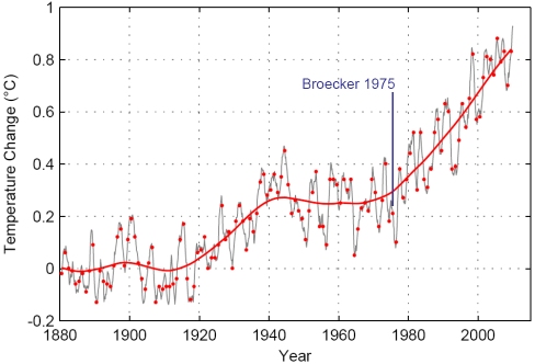
Global warming is turning 35! Not only has the current spate of global warming been going on for about 35 years now, but also the term “global warming” will have its 35th anniversary next week. On 8 August 1975, Wally Broecker published his paper “Are we on the brink of a pronounced global warming?” in the journal Science. That appears to be the first use of the term “global warming” in the scientific literature (at least it’s the first of over 10,000 papers for this search term according to the ISI database of journal articles).

In this paper, Broecker correctly predicted “that the present cooling trend will, within a decade or so, give way to a pronounced warming induced by carbon dioxide”, and that “by early in the next century [carbon dioxide] will have driven the mean planetary temperature beyond the limits experienced during the last 1000 years”. He predicted an overall 20th Century global warming of 0.8ºC due to CO₂ and worried about the consequences for agriculture and sea level.

Global temperature up to June 2010 according to the NASA GISS data. Grey line is the 12-month running average, red dots are annual-mean values. The thick red line is a non-linear trend line. Broecker of course did not have these data available, not even up to 1975, since this global compilation was only put together in the late 1970s (Hansen et al. 1981). He had to rely on more limited meteorological data.

To those who even today claim that global warming is not predictable, the anniversary of Broecker’s paper is a reminder that global warming was actually predicted before it became evident in the global temperature records over a decade later (when Jim Hansen in 1988 famously stated that “global warming is here”).

Broecker is one of the great climatologists of the 20th Century: few would match his record of 400 scientific papers, a full sixty of which have over 100 citations each! Interestingly, his “global warming” paper is not amongst those highly-cited ones, with “only” 79 citations to date. Broecker is most famous for his extensive work on paleoclimate and ocean geochemistry.

It is very instructive to see how Broecker arrived at his predictions back in 1975 – not least because even today, many lay people incorrectly assume that we attribute global warming to CO₂ basically because temperature and CO₂ levels have both gone up and thus correlate. Broecker came to his prediction at a time when CO₂ had been going up but temperatures had been going down for decades – but Broecker (like most other climate scientists at the time, and today) understood the basic physics of the issue.

Basically his prediction involved just three simple steps that in essence are still used today.

Step 1: Predict future emissions

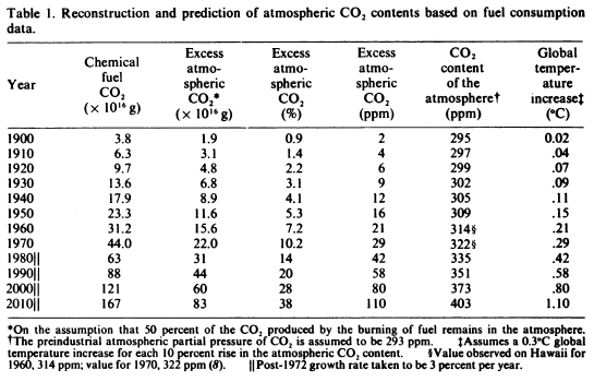
Broecker simply assumed a growth in fossil fuel CO₂ emissions of 3% per year from 1975 onwards. With that, he arrived at cumulative fossil CO₂ emissions of 1.67 trillion tons by the year 2010 (see his Table 1). Not bad: the actual emissions turned out to be about 1.3 trillion tons (Canadell et al, PNAS 2007 – estimate extended to 2010 by me).

A shortcoming, from the modern point of view, is that Broecker did not include other anthropogenic greenhouse gases or aerosol particles in his calculations. He does however discuss aerosols, which he calls “dust”. In fact, the first sentence of the abstract (quoted above) in full starts with an if-statement:

If man-made dust is unimportant as a major cause of climate change, then a strong case can be made that the present cooling trend will, within a decade or so, give way to a pronounced warming induced by carbon dioxide.

That is a nod to the discussion about aerosol-induced cooling in the early 1970s. Broecker rightly writes:

It is difficult to determine the significance of the next most important climatic effect induced by man, “dust”, because of uncertainties with regard to the amount, the optical properties and the distribution of man-made particles,

citing a number of papers by Steve Schneider and others. Because he cannot quantify it, he leaves out this effect. Here luck was on Broecker’s side: the warming by other greenhouse gases and the cooling by aerosols largely cancel today, so considering only CO₂ leads to almost the same radiative forcing as considering all anthropogenic effects on climate (see IPCC AR4, Fig. SPM.2).

Table 1 of Broecker (1975)

Step 2: Predict future concentrations

To go from the amount of CO₂ emitted to the actual increase in the atmosphere, one needs to know what fraction of the emissions remains in the air: the “airborne fraction”. Broecker simply assumed, based on past data of emissions and CO₂ concentrations (Keeling’s Mauna Loa curve), that the airborne fraction is a constant 50%. I.e., about half of our fossil fuel emissions accumulates in the atmosphere. That is still a good assumption today, if you look at the observed CO₂ increase as fraction of fossil fuel emissions. Broecker calculated that about 35% of the emissions is taken up by the ocean and the other 15% by the biosphere (again not far from modern values, see Canadell et al.). On this basis he argued that if the ocean is the main sink, the airborne fraction would remain almost constant for the decades to come (his calculations extend to the year 2010).

Thus, with a 3% increase in emissions per year and 50% of that remaining airborne, it is easy to compute the increase in CO₂ concentrations. He obtains an increase from 295 to 403 ppm from 1900 to 2010. The actual value in 2010 is 390 ppm, a little lower than Broecker estimated because his forecast cumulative emissions were a little too high.

Step 3: Compute the global temperature response

Now we come to the temperature response to increased CO₂ concentration. Broecker writes:

The response of the global temperature to the atmospheric CO₂ content is not linear. As the CO₂ content of the atmosphere rises, the absorption of infrared radiation will “saturate” over an ever greater portion of the band. Rasool and Schneider point out that the temperature increases as the logarithm of the atmospheric CO2 concentration.

Based on this logarithmic relationship (still valid today) Broecker assumes a climate sensitivity of 0.3ºC warming for each 10% increase in CO2 concentration, which amounts to 2.2ºC warming for CO₂ doubling. This is based on early calculations by Manabe and Wetherald. Broecker writes:

Although surprises may yet be in store for us when larger computers and better knowledge of cloud physics allow the next stage of modeling to be accomplished, the magnitude of the CO₂ effect has probably been pinned down to within a factor of 2 to 4.

The AR4 gives the uncertainty range of climate sensitivity as 2-4.5ºC warming for CO₂ doubling, so there still is about a factor of 2 uncertainty and Broecker used a value near the very low end of this uncertainty range. Modern estimates are not only based on model calculations but also on paleoclimatic and modern data; the AR4 lists 13 studies that constrain climate sensitivity in its table 9.3.

In Broecker’s paper the warming calculated with the help of climate sensitivity happens instantaneously. Today we know that the climate system responds with a time lag due to ocean thermal inertia. By neglecting this, Broecker overestimated the warming at any given time; accounting for thermal inertia would have reduced his warming estimate by about a third (see AR4 Fig. SPM.5). But again he was lucky: picking ~2ºC rather than the more likely ~3ºC climate sensitivity compensates roughly for this, so his 20th-Century warming of 0.8ºC is almost spot on (the actual estimate being closer to 0.7ºC, see Fig. above). (A modern version of this back-of-envelope warming calculation is found e.g. in our book Our Threatened Oceans, p.82.)

Natural Variability

Broecker was not the first to predict CO₂-induced warming. In 1965, an expert report to US President Lyndon B. Johnson had warned: “By the year 2000, the increase in carbon dioxide will be close to 25%. This may be sufficient to produce measurable and perhaps marked changes in climate.” And in 1972, a more specific prediction similar to Broecker’s was published by the eminent atmospheric scientist J.S. Sawyer in Nature (for a history in a nutshell, see my newspaper column here).

The innovation of Broecker’s article – apart from introducing the term “global warming” – was in combining estimates of CO₂ warming with natural variability. His main thesis was that a natural climatic cooling

has, over the last three decades, more than compensated for the warming effect produced by the CO₂ [....] The present natural cooling will, however, bottom out during the next decade or so. Once this happens, the CO₂ effect will tend to become a significant factor and by the first decade of the next century we may experience global temperatures warmer than any in the last 1000 years.

The latter turned out to be correct. The idea that the small cooling from the 1940s to 1970s is due to natural variability still cannot be ruled out, although more likely this is a smaller part of the explanation and the cooling is primarily due to the “dust” neglected by Broecker, i.e. due to the rise of anthropogenic aerosol pollution (Taylor and Penner, 1994). However, the way Broecker estimated and even predicted natural variability has not stood the test of time. He used data from the Camp Century ice core in Greenland, arguing that these “may give a picture of the natural fluctuations in global temperature over the last 1000 years”. Ironically, Broecker’s own later work on Atlantic ocean circulation changes showed that Greenland is likely even less representative of global temperature changes than most other places on Earth, it being strongly affected by variability in ocean heat transport (see our recent post on the Younger Dryas, or Broecker’s latest book The Great Ocean Conveyor). However, Broecker was right to conclude that the buildup of CO₂ would sooner or later overwhelm such natural climate variations.

Overall, Broecker’s paper (together with that of Sawyer) shows that valid predictions of global warming were published in the 1970s in the top journals Science and Nature, and warming has been proceeding almost exactly as predicted for at least 35 years now. Some important aspects were not understood back then, like the role of greenhouse gases other than CO₂, of aerosol particles and of ocean heat storage. That the predictions were almost spot-on involved an element of luck, since the neglected processes do not all affect the result in the same direction but partly cancel. Nevertheless, the basic fact that rising CO₂ would cause a “pronounced global warming”, as Broecker put it, was well understood in the 1970s. In a 1979 TV interview, Steve Schneider rightly described this as a consensus amongst experts, with controversy remaining about the exact magnitude and effects.

Reference
BROECKER WS, 1975: CLIMATIC CHANGE – ARE WE ON BRINK OF A PRONOUNCED GLOBAL WARMING?
SCIENCE Volume 189, Pages 460-463.

Nanotech Coating Produces Electricity From Sewage

http://www.dailytech.com/Nanotech+Coating+Produces+Electricity+From+Sewage/article19130.htm

Could change the face of wastewater treatment

Oregon State University engineers haveapplied new coatings on anodes of microbial electrochemical cells, which heightens their electricity production by 20 times, and is another step closer to producing electricity from sewage. 

The graphite anodes were coated with palladium at one point in order to produce electricity, but that didn't produce quite as much as the nanoparticle layer of gold, which is what increased the electricity production by about 20 times. This is a huge advance toward technology that could both produce levels of electricity and clean biowaste at the same time, ultimately changing the face ofrenewable energy and wastewater treatment. Also, this sort of technology could help treat wastewater in developing nations where an inadequate power supplyprevents proper treatment.

During the course of these experiments, researchers inserted bacteria from sewage into an anode chamber and allowed it to form a biofilm, absorb nutrients and grow. The bacteria releases electrons during this process and fuels electricity production. 

"This is an important step toward our goal," said Frank Chaplen, an associate professor of biological and ecological engineering. "We still need some improvements in design of the cathode chamber, and a better understanding of the interaction between different microbial species. But the new approach is clearly producing more electricity." 

In addition, researchers have reason to believe that an iron nanoparticle coating would increase the electrical output of sewage as much as the layer of gold in some types of bacteria. Also, a "similar approach" could produce hydrogen gas rather than electricity, which could lead to further advancements in hydrogen fuel cell technology for cars as well as treating wastewater. 

"Recent advances in nanofabrication provide a unique opportunity to develop efficient electrode materials due to the remarkable structural, electrical and chemical properties of nanomaterials," said the published research paper. "This study demonstrated that nano-decoration can greatly enhance the performance of microbial anodes."

While more research is required to lower costs and improve efficiency, researchers say this technology has been proven in the laboratory. The study was led by Hong Liu, an assistant professor of biological and ecological engineering, and was published in Biosensors and Bioelectronics.